Similar to the concept of splicing graphs [Heber 2002], we employ a graph structure for representing the reference transcriptome that is quantified in a non-redundant data structure. Each edge
represents a segment of an annotated pre-mRNA molecule by the genomic coordinate of the corresponding 3'-tail and 5'-head position, by the type (exonic or intronic), and by the set
of supporting transcripts (Definition 1).
Definition 1 (Segment Graph Properties): two adjacent edges in G are characterized by:
(i) they share the same intermediary splice site (adjacency)
(ii) they describe the exon-intron structures of all transcripts spanning s (completeness)
(iii) they either differ in mode or in supporting transcripts (discrimination)
To ensure the properties of at the respective transcript edges, all transcription initiation sites are connected to an artificial source node, and all cleavage sites are connected to an artificial sink node [Sammeth 2008]. Once the segment graph
has been constructed for a locus, the edge set E describes the backbone of exonic segments and introns from the 3'-most transcription start to the 5'-most cleavage site, with additional introns, source and sink links that allow to navigate alternative transcripts (Fig.1, panel A and B).
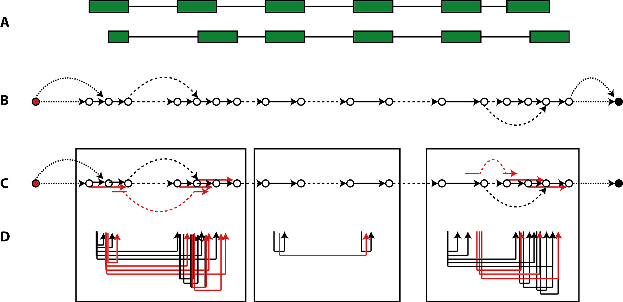
Figure 1: segment graph inferred on an alternatively spliced locus. (A) The exon-intron structure of a locus with two alternative transcripts. (B) Segment graph elements with links by exonic edges shown as solid arrows, links by intronic edges as dashed arrows, and source/sink links as dotted arroes. (C) Expansion of the segment graph by super-edges coalesced from adjacent exon segments or from splice junctions. (D) Super-edges formed by paired-end mappings within the bounds of the three windows marked, to keep (super-) edge combinations within graphical resolution bounds.
Overview
Content Tools